As a Canadian and a life-long fisherman, I have spent some time on the water. In 2018, for the tail-end of my MSc program in Water Resources Engineering at the Vrije Universiteit Brussel, I had to pick a thesis project for which I would do some science and write my first paper. Among the list of topics, “Is lake ice disappearing from the Earth System?” hooked me. I ignored the technical implications of the project summary, which included something about ISIMI and its lake sector, some lake models and climate models, and a high performance computer or two. Instead, my internal dialogue went: “I fish. And we have a lot of fun on the ice at home” (Figure 1). After 3-years of work that included a lot of self-taught programming, reading detection and attribution studies and coordinating with an international group of 20 researchers (without whom this wouldn’t be possible), this eventually led to a paper that established a “yes” to the title of this article.
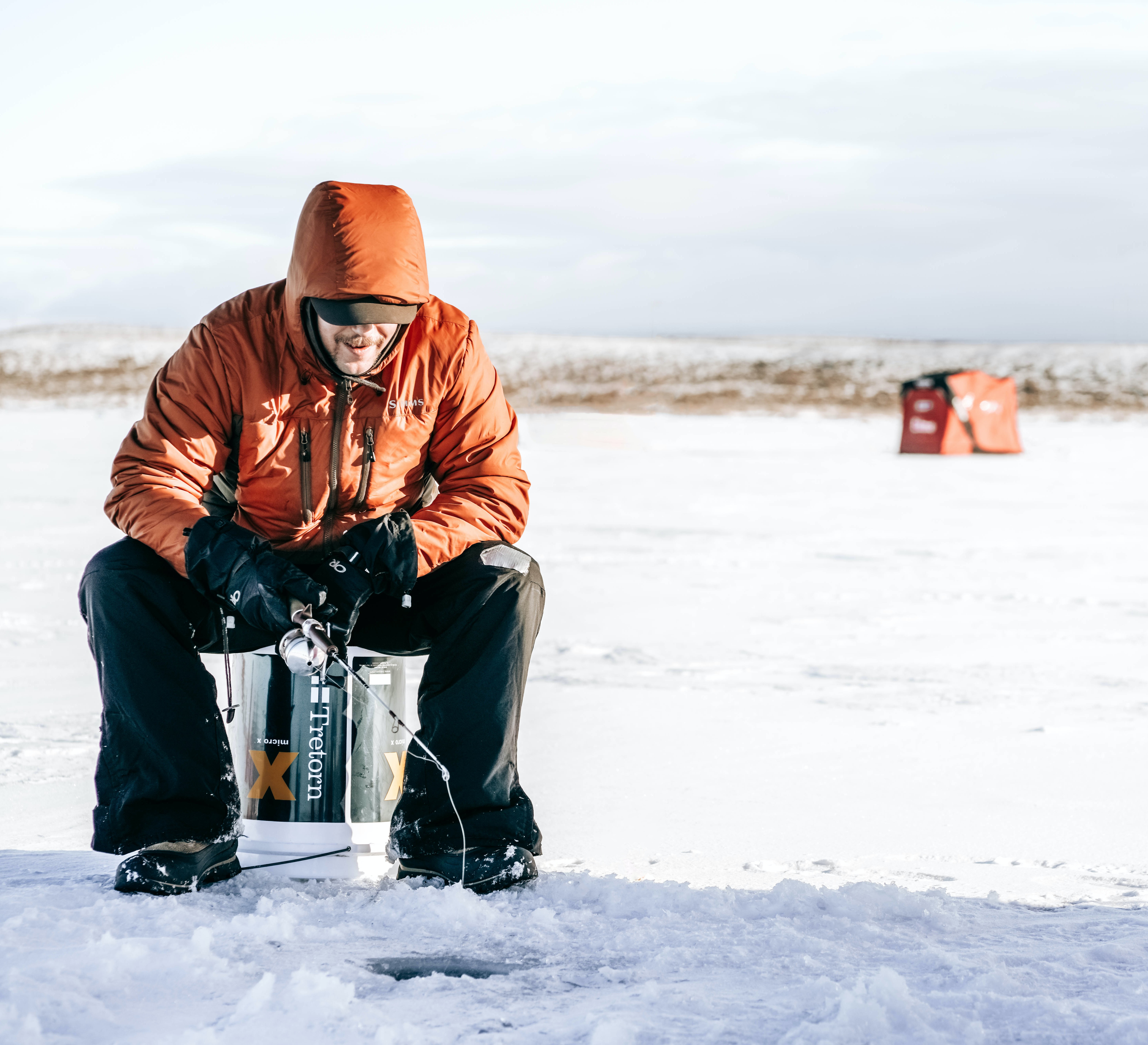
Ice-fishing with a rod and ice shanty in the background. Note that this is not me.
FIG 1 / Picture by Glenna Haug
But if you do not participate in redneck stuff “on the water,” why should you care about whether lakes are warming and losing their ice?
Lakes provide us with ecosystem services that we can estimate a monetary value for. Ecosystem services are benefits accrued by humanity from well-functioning ecosystems. For lakes, this includes recreational and subsistence activities. Among the latter, drinking water supply, aquaculture, commercial and subsistence fishing are important human-lake interactions that are widely dependent on in both developing and developed countries.
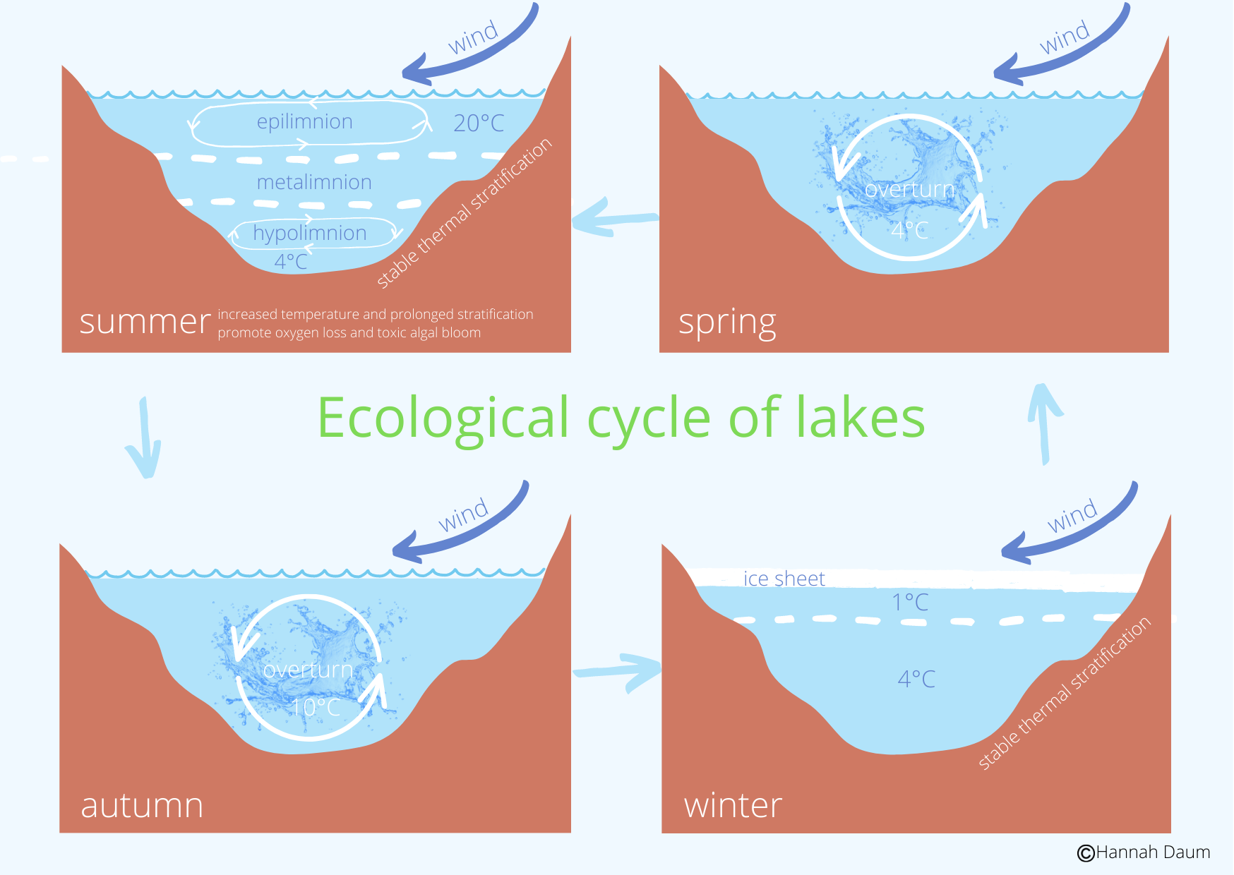
Unmitigated and rapid changes to lake physical characteristics, such as water temperature and lake ice cover, can jeopardize these ecosystem services. This is rooted in how these characteristics are foundational to the lake environment. Lake ice cover acts as a seasonal barrier to heat, oxygen and particulates. The timing of lake ice onset and breakup therefore controls the seasonality by which lake thermal layers can turn over and mix, and, in between these mixing events, when they stratify by temperature and density. These mixing and stratification periods become a cascade for the activity of lake biota by establishing nutrient availability and providing the thermal habitats that organisms are adapted to (see Figure 2). Therefore, in a warming climate, lakes could incur physical changes with increased temperature and prolonged stratification that are unsuitable for existing species (Kraemer et al. 2021) but which promote lake oxygen loss (Jane et al. 2021) and acute events like toxic algal blooms (Posch et al. 2012).
If lakes are important and their ecosystems are sensitive to warming, how would you prove whether or not climate change has already affected them?
When we observe shifts or trends in a subset of the earth system - be it our oceans, rivers, lakes or local atmospheric conditions - we might identify the direction of this change as agreeing with its expected pathway under a) rising greenhouse gas emissions and resultantly b) a (mostly) warmer climate. For example, perhaps you observe that the winter ice cover on your local fishing lake hasn’t lasted as long into March as it did when you were a child. Under a warming climate, this makes sense: in theory, you can causally link your observation to climate change. However, while these experiential changes might truly be local features of the broader strokes of climate change, you haven’t proved this numerically or statistically. In a statistical sense, questions remain over other probable explanations for the phenomenon you’ve witnessed. Perhaps this lesser ice cover is due to chaotic “swings” in the climate – internal climate variability – bringing warmer temperatures or less snow for amassing ice thickness?
Since there exists some need to dissect what we observe from what is plausible via natural variations in weather, we turn to the Intergovernmental Panel on Climate Change’s Working Group I (IPCC WGI) detection and attribution framework (Bindoff et al. 2013; Field et al. 2014; Hegerl et al. 2007). The complementary approach to attribution of Working Group II addresses the separation of climate change versus additional human drivers and is explained in detail in the ISIpedia-article “How much of this change is due to climate change?”.
The goal of a trend detection and attribution analysis is to prove the role of human caused climate change in affecting some observed variable of interest (e.g. global mean temperature, or river discharge), which we will call the target variable (Figure 3). Detection and attribution can also help explain the roles of different climate forcings in a shifted target variable (Figure 3, panel b). External forcings of interest that can be largely driven by human influences include greenhouse gas and aerosol emissions and land cover change. These are sometimes compared to a lumped set of natural external forcings, including volcanic and solar activity. The expected effect of a given forcing – or group of forcings – on the target variable is described as a fingerprint, which can be understood as a space-time pattern of change in the target variable (Figure 3, panel b). However, we don’t have a second Earth to run controlled, planet-scale experiments to test these fingerprints in the real world. Rather, we estimate them with numerical simulations from general circulation models (GCMs). A detection and attribution analysis therefore requires separate datasets of the target variable; those that are observationally-based and contain some pattern whose origin you want to explore, and fingerprints simulated by models with different combinations of forcings. The presence of model-simulated fingerprints is evaluated in the observations to prove their influence in a 2-step process.
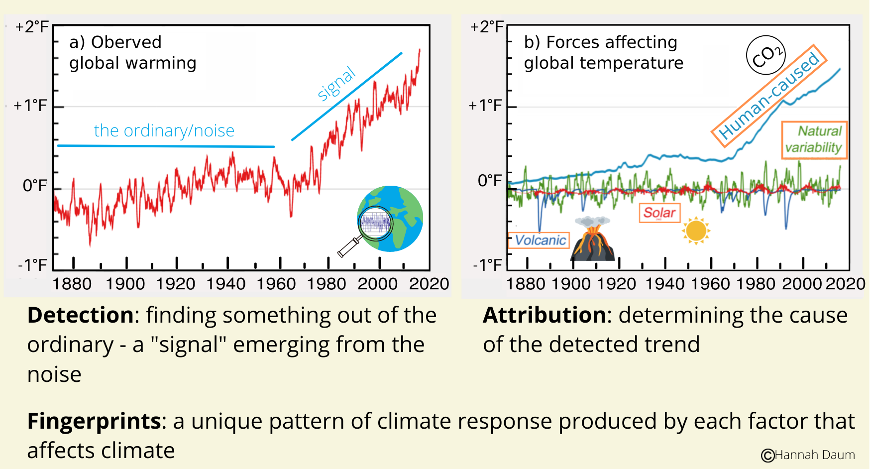
Following IPCC WG I, step 1, “detection,” is demonstrating whether or not observed changes are significant. Significance here asks the following: can you prove that these changes are distinguishable from their likely range under internal climate variability, or, in other words, that the probability of these changes occurring under internal climate variability is sufficiently small? This is done by comparing observations against simulations of a pre-industrial climate, which captures the distribution of possible changes in the target variable that are within their internal variability and not contaminated by the external forcings described above (Figure 3, panel a).
Upon detecting a signal in your target variable, there remains uncertainty in what fingerprint was dominantly present in the observed shift, or, in other words, which forcing caused this significant change. Establishing this link with some level of statistical confidence is step 2, “attribution.” Attribution is technically more difficult, as it requires multiple lines of evidence for confidently establishing the suspect forcing behind your observed changes. This is done by simultaneously demonstrating two things. First, that observed changes are consistent with the fingerprints whose forcings you hypothesized are responsible. Here, hypothesized agents are typically one of the external forcings from human influences from earlier. And second, demonstrating inconsistencies between observed changes in the target variable and other possible combinations of external forcings excluding those hypothesized as responsible.
This generalized description of detection and attribution requires a translation to the context of assessing signals in lake physics. The description of detection and attribution above reflects the definition of IPCC WG I. The effects of climate change forcings on meteorological variables are assessed against the backdrop of internal climate variability. Here, one might attempt to detect the change in precipitation or near surface temperature and then attribute these to human influences. In our study we take it one step further and assess lake variables that are changing as a result of meteorological characteristics directly affected by greenhouse gas or aerosol emissions. Technically, we assess lake signals in the same way as it is done for meteorological variables in the WGI framework; by substituting climate model simulations under different forcings for lake model simulations driven by climate model simulations under different forcings.
Setting up our lake analysis with observations and ISIMIP simulations
So, in order to make confident assessments of the influence of climate change on lakes, we require quite some information on lake systems. Unfortunately, there are roughly 117 million lakes on earth (Verpoorter et al. 2014). While limnologists have been generating in situ lake temperature and ice phenology datasets, in aggregate these are not sufficiently spatially representative for global studies. They also do not cover enough time to span a change in climatology, which normally requires 30-50 years of data. The same space-time limitations can be true for satellite-based observations as well.
To overcome the limitations of true observational data for evaluating the world-wide signal of climate change impacts on lakes, global lake simulations are a reasonable compromise. In our study, we did not directly use in situ or satellite observations for detection and attribution. Instead, we use lake reanalysis simulations in their place (see timing and temperature). As this is a far leap from scientists in boats recording temperatures, we evaluated the reanalysis dataset against observations from the European Space Agency (ESA) and other sources, finding that the reanalysis adequately captured the trends of these additional observed datasets. For the sake of consistency with the detection and attribute explanation, we’ll hereby refer to the reanalysis dataset as the observations.
What aspects of lakes do we assess?
Our detection and attribution analysis focuses on a few key lake variables in the observations and model datasets that capture important aspects of lake physics. First we assess near-surface lake temperatures at 2-meters depth, which we’ll hereby refer to as lake temperature. This was chosen as a balance point between assessing deeper temperatures, which could be unreliably simulated at this scale, and surface temperatures, which would too directly reflect air temperature. This choice is also compatible with our observations. Where the observations report mixed layer temperatures, it is a safe assumption that the modeled 2-meter temperatures will be encompassed by the vertical extent of lake mixed layers, which are the uppermost sections of lakes that exhibit uniform temperatures because of mechanisms driving mixing (Figure 2, see “epilimnion” in the summer panel). The chosen depth is also ideal in that it is comparable against observational data used in the aforementioned trend evaluation with satellite and in-situ sources. For ice cover, we computed ice onset, breakup and duration indices from ice thickness data. We found this ideal in comparison to analyzing the signal in ice thickness because ice thickness may respond to climate change in a more complicated manner. As well, because observations for ice thickness are less available for validating reanalysis ice thickness. Finally, the detectability of ice onset versus breakup signals pushes a more profound message about how the seasonality of lake mixing events is being shifted (see Figure 2). For all of these variables, we take their global means to represent lake changes world-wide in our analysis.
Our observations for ice cover in the study period can be seen in this interactive figure. Here we see, for example, that ice onset dates are the least impacted of the three ice indices; the dates at which ice begins occur at moderately later times in most of the northern hemisphere (panel a). However, in Germany and Poland, for example, lakes in our observations have shifted their first day of ice cover further into the Winter season by 10 to 20 days. It is also clear that changes in ice break-up dates have been more sensitive to historical climate change (panel b), albeit with a hiatus in impacts in eastern Canada. Here, lakes across Scandinavia and Russia are losing seasonal ice cover earlier in the Spring by 5-20 days. Finally, these impacts sum in the ice duration outlook (panel c), causing substantial changes in ice cover in much of eastern Europe.
We also show here the changes in seasonal lake mixed layer temperatures in our observations. Here, lake temperatures warm notably in the summer season in upper latitudes, increasing by 1.5 to 2.5 ℃ in eastern Russia. For the rest of the seasons, historical changes in lake mixed layer temperatures are less disturbed.

Our model simulations come from the namesake of this platform, the lake sector of the Inter-sectoral Impact Model Intercomparison Project (ISIMIP). At the time of our analysis, the lake sector included simulations from 5 lake models using boundary conditions from 4 GCMs under pre-industrial, historical and future climates of varying emissions scenarios (RCP 2.6, 6.0 and 8.5). One should imagine each realization inside this ensemble of datasets – take, for example, the historical period simulated by the lake model “SIMSTRAT-UoG” under the forcing of the GCM “MIROC5” – as providing global, daily, gridded fields of information on the vertical temperature profile and ice thickness of “representative lake” grid cells where real lakes exist. We use these ensembles of simulations from different models in hope of including model structural uncertainties in our analyses. This means that, as each of the lake models takes a different approach to producing lake temperature profiles and ice cover, the models estimate a range of possible values, resulting in uncertainties about the true changes in lakes that these simulations attempt to describe. The same is true of the GCMs that force the lake models. By including results across a breadth of model patterns, we are able to more transparently assess uncertainties in our lake projections.
Detecting changes in lake temperature and ice cover using a correlation-based approach
We start our detection and attribution analysis with a correlation approach. The idea here is to establish a range of possible lake trends that could occur in a pre-industrial climate and see how our observed lake trends compare to this. We do this with 3 sets of data. The first is our lake model simulations forced by pre-industrial climate runs (in our figures this is PIC), which span 439 years (1661-2099). These only reflect the influences of internal climate variability on lakes and therefore aren’t logically tied to specific periods of human influence. With this in mind, we can freely extract as many “chunks” of pre-industrial time-series as possible that match the 39-year length of our observations (covering 1981-2019) that we want to compare to. This yields a large sample of 39-years time series of pre-industrial lake data across all our lake model/climate model combinations, characterizing the limits of lake behaviour under internal climate variability in the time frame of our observations. Second, we compute the estimate of the combination of the various human and natural forcings that best reflects observed lake changes for 1981-2019, which is the multi-model mean fingerprint from historical lake simulations (HIST). Third is our observed changes in each lake variable (OBS).
For each pre-industrial control chunk (PIC), we compute its correlation with the multi-model mean historical fingerprint (HIST). This re-communicates the range of possible lake behaviours under internal climate variability as a distribution of correlations, as illustrated by the grey bars in Figure 6, first panel. Typically, datasets are de-trended before computing their correlation coefficients. This is to avoid capturing the spurious likenesses between the two datasets based on their overall matching trajectory in exchange for the typical intention of a correlation, which is to focus on their joint variability. However, in our study we do not remove the trends in our data. Rather, we want to capture them in the correlations to represent potential lake changes through the influences of either a) climate change in the models and observations or b) internal climate variability in the pre-industrial control chunks. We then compute a final correlation between the observations (OBS) and our best estimate of human and natural forcings, i.e. the historical fingerprint (HIST), as represented by the vertical red line in Figure 6. We use the position of this correlation relative to the distribution of pre-industrial correlations (PIC) to understand how unlikely it is that the observed patterns of lake change match what is possible through internal climate variability. If this correlation is well within the distribution of pre-industrial correlations, the observed lake changes are likely to be only influenced by internal climate variability. The more the correlation of observations is out of this distribution, the higher the likelihood that observed changes are influenced by external forcings. For all lake variables, this correlation between the observations and historical fingerprints is strong and sits in the range of very low probability outcomes from internal climate variability (Figure 6; first panel). Using the definitions from earlier, this analysis yields a detection of changes in lake temperature and ice cover as it clarifies that the patterns in our observations are distinct from what is possible from internal climate variability.
Detection and attribution with Regularized Optimal Fingerprinting
Most trend detection and attribution practices take on the general form of regressing observed changes onto model-simulated fingerprints to assess the presence of these fingerprints in the observations. Recall that fingerprints are space-time patterns of change in the target variable due to a certain forcing, or a combination of forcings. After fitting the regression, you have achieved some regression parameters, which are mostly called scaling factors, that scale the fingerprints to fit the observations. These scaling factors establish detection and attribution by communicating the presence of the fingerprints in the observations. In other words, we are dissecting observed patterns of change as a sum of their scaled fingerprints for different forcings. This assumes that the fingerprints are a) reliable estimations of their occurrence in reality (which can be tough to chew on) and b) linearly additive. For example, in looking at observed changes in surface temperatures, you would therefore assume that the simulated fingerprint of natural forcings can be reliably summed with the fingerprint of greenhouse gases to achieve their cumulative effect on surface temperatures. In essence, this is what Regularized Optimal Fingerprinting (ROF) performs.
The statistics behind what is “regularized” and what is “optimal” in ROF are outside the scope of this communication, yet, some other details need to be described. Specifically, the ways in which these scaling factors tell us about detection or attribution. First, this exercise operates under the null hypothesis that the effect of each fingerprint is insignificant or indistinguishable from internal climate variability. In the regression context, this means that the scaling factors overlap with 0. So, when a fingerprint has a significant influence on the observations and contributes to the observed pattern of change, its scaling factor is non-zero and we reject the null hypothesis. Subject to the earlier conditions that this is only the case for the hypothesized forcings responsible and not for remaining combinations of forcings, strict attribution can be achieved when the scaling factors are consistent with 1.
Here comes a debatable caveat in our study; we only had the full historical fingerprint at our disposal. Our lake simulations did not include runs driven by a natural set of historical forcings that, in combination with the full historical forcings, could isolate anthropogenic influences in ROF. This means that any successful attribution we claim from computing scaling factors consistent with 1 only technically demonstrates - in addition to detection - that observed changes are attributed to all external forcings, both natural and human-based. However, in light of a breadth of attribution studies that clearly show the dominant role of greenhouse gas emissions in historical temperature changes (Myhre et al. 2013), we argue that attribution to the full suite of historical forcings still proves the imprint of human influence.
As with the correlation analysis, we undertake ROF with global average series’ for lake temperatures and lake ice cover. This analysis confirms the detection results of the correlation approach, with each scaling factor being non-zero. We further attribute, under the caveat above, all three ice indices to human influences. We do not attribute lake temperature changes, as the models appear too sensitive here and produce a strong positive bias in temperature trends.
Takeaway
Our study demonstrates that it is extremely unlikely that historical lake changes have occurred due to pre-industrial climate variability. We form a strong argument that these changes are caused by human influences on the climate. Future improvements to our work could be achieved in a number of ways. First, using true observational reference products (Verpoorter et al. 2014) directly in an attribution framework would better establish the message of worldwide lake changes, yet this is not possible until these datasets grow in global coverage and time span. Second, properly ruling out the influences of natural external climate forcings on historical lake changes, which would require lake simulations under a natural historical set of forcings, would further improve our confidence in these findings. Despite these shortcomings, our findings communicate yet another set of systems already impacted by climate change that underline the need for mitigation.