Is the observed positive trend in global flood damages due to climate change?

We already see effects of climate change in rainfall patterns - but can we also see it in flood damage?

You can think of basically three reasons for trends in observed flood induced damages: it could be a trend in the magnitude or frequency of flooding (hazard), a change in asset distributions (exposure) or a change in the susceptibility of the assets when exposed to flooding (vulnerability; Figure 2).

---

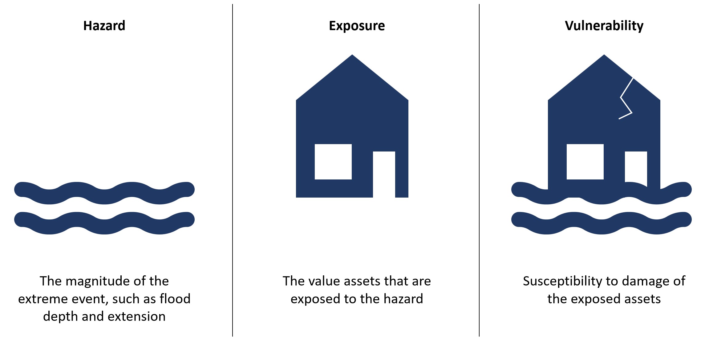
Hazard encompasses all factors that contribute to the magnitude of the flood. These factors are the atmospheric conditions (precipitation, evaporation), the catchment conditions (e.g. soil sealing through urbanisation) and the changes in the river channel (e.g. through river regulation and dams). Exposure describes the value that is exposed to the hazard for example the value of all houses that are flooded or the number of people that live in the flooded area. Vulnerability defines how much of the exposed value is destroyed when hit by a disaster. Vulnerability depends e.g on how people are prepared for disasters (e.g through early warning systems), how well they are protected (e.g. through dikes) or on how robust their building infrastructure is (e.g. building material). These three components determine how much damage is caused by a disaster and all of them can change over time and lead to a change in the long-term damage trend.

---

FIG 2

Previous studies concluded that the increase in damage is mainly caused by population and economic growth that have led to higher exposed value in flood prone areas (Neumayer and Barthel 2011; Kundzewicz et al. 2014). On the other hand, the trends in disaster damages seem to be smaller than those in economic and population growth, suggesting that people have also improved protection levels over time, for example by building dikes or moving out of flood prone areas.

Why is there no obvious climate signal in flood damages?

Our paper addresses the hypothesis that the change in hydrological conditions is too diverse across different regions to become visible on global or continental scale. Effects of changing climate have led to increasing river flow maxima in some regions and decreasing maximum flows in others (Figure 3a). Thus aggregating across regions while ignoring these differences may mean that diverging trends in flood damages are leveled out.

This has not been systematically addressed so far because most studies attributing changes in flood induced damages) have focussed on changes in vulnerability rather than changes in the climate-related hazards (Formetta and Feyen 2019; Jongman et al. 2015; Tanoue, Hirabayashi, and Ikeuchi 2016). In these cases damages were usually aggregated across regions with similar socio-economic conditions, e.g high, medium or low income countries, as it is assumed that vulnerability may change homogeneously across these areas.

As we were interested in the effect of climate change we decided to identify regions with similar trends in hazards using changes in annual maximum river discharge (see Figure 3a). Global analyses of river discharge indicate that even within the same world region annual maximum discharge has increased in some areas while it has decreased in others (Do, Westra, and Leonard 2017; Gudmundsson et al. 2019). To identify regions where discharge trends have increased and those where it decreased, we cannot rely on observational data because gauge stations are very unevenly distributed across the globe and data availability is sparse for most areas in the world. To overcome this issue, we have to use the output from hydrological and river routing models instead. These models use observed weather data for the last four decades to generate river discharge on a 0.25 x 0.25 degree resolution (Figure 3a). Based on the output of these models, we estimate a trend for annual maximum discharge in each river basin. For example in Latin America, annual maximum river flows have decreased in the light green basins, but increased in the dark green basins (Figure 2b). We use river basins as regional units and combine them to subregions of basins showing a positive discharge trend (R₊) and of basins with a negative trend (R_-) e.g. for Latin America, comprising all river basins with increasing trend (LAM₊) and all river basins with decreasing trends (LAM_-). When it comes to damage assessment we sum up all the damage that occurs in these subregions.

---

Absolute trends in annual maximum daily discharge in the time period 1971-2010, model output from the full ensemble of hydrological models driven with observed weather coupled with CaMa-Flood. b Map of the nine geographical world regions: North America (NAM), Eastern Asia (EAS), Europe (EUR), Latin America (LAM), Central Asia & Russia (CAS), South & Sub-Saharan Africa (SSA), South & South-East Asia (SEA), North Africa & Middle East (NAF), Oceania (OCE) chosen according to geographical proximity and similarity of socio-economic structure. These regions are then further divided into subregions assembled of river basins with positive (R₊, dark colors) and negative discharge trends (R_-, light colors).

---

FIG 3 / Image source: Sauer et al. (2021)

Development of a model of flood damages

An alternative world where exposure and vulnerability remain unchanged, while climate change has increased cannot be observed. Therefore, we need to simulate a world where we can keep individual drivers of flood damage constant to estimate the effects of the others. Such a model needs information about historical flood extents and depth, an approximation of historical changes in asset distributions and a way to derive changes in vulnerability from observed damages as there is no direct access to information about vulnerabilities on global scale. So this is how we have built a model to understand the drivers of historical flood induced damages.

2. Estimating potential damages accounting for changes in exposure

To derive the potential damage induced by the simulated historical flooding we combine the information about flood extent (more info) (X % of a grid cell flooded at least once within a given year) with annual maps of asset distributions (10km x 10km resolution) derived from national economic development and changes in population distribution (more info).

We assume that there is a temporally constant flood protection to a certain level available from the FLOPROS database (Scussolini et al. 2016). This database provides an estimate of the flood protection expressed in return periods (e.g. there is flood protection against 100 year events) for each province. In the best case this is the actually implemented protection. If this is not available the protection level is taken from defined policy levels and if this is not given either, the protection level is estimated from the given income level of the province. In our modeling we assume that there is no flooding if the protection level is not exceeded. When the protection level is exceeded we assume that flooding takes place as if there was no protection. In addition, we assume that assets are uniformly distributed within each grid cell. The assets are fully destroyed at flood heights higher than 12 meter and not destroyed at zero flood depth with a smooth function in between (see Figure 4). This highly simplified assumption about vulnerability does not vary with time. As there is no direct information about the temporal variation in vulnerability it is derived by comparing the potential damage derived here to the actual reported damages provided by Munich Re as described in the next section.

---

Fraction of the asset value (0-1) that is destroyed at varying flood depth, in any case the maximum damage is reached at a flood depth of 12 m.

---

FIG 4 / Image source: Sauer et al. (2021)

3. Estimation temporal changes in vulnerability

To estimate the long-term temporal development of vulnerability we compare the annual potential damage estimated for each sub-region to the reported damage (see red dots in Figure 5 for the global region with increasing discharge and decreasing discharge, respectively). Assuming that vulnerability only changes slowly over time rather than showing strong annual fluctuations we fit a smooth line to these dots and apply the associated annual fraction to the estimated potential damage to simulate damage by our full model while accounting for change in climate, exposure and vulnerability. All the modeling components are then put together in the open source impact modeling framework CLIMADA. See also the corresponding code repository which support the article findings with valuable demonstration examples and full implementation instructions and code.

---

Estimated vulnerability change over time for a the entire globe (GLB), b all the basins of the world with increasing discharge maxima (GLB₊) and c all the basins of the world with decreasing discharge maxima (GLB_-). To account for changes in vulnerability over time in our model we multiply the potential damage with the time dependent vulnerability factor shown here as black line. This is the smoothed ratio of observed damage (DObs) and the simulated potential damage.

---

FIG 5 / Image source: Sauer et al. (2021)

How good is the model? Is our tool accurate enough to address the attribution question?

Figure 6 shows the reported global damage for the entire globe and for its subregions of increasing and decreasing discharge in comparison to the damages simulated by our full model. Well, the agreement is not perfect, but given a range of limitations of the global hydrological simulation, missing detail in the knowledge of asset distributions and potential errors of reported damages we consider it a quite good agreement if at least 20% of the variation in reported damages can be explained. In particular the observed trend in damages is quite well reproduced (see purple bar compared to black empty bar in the right panels).

---

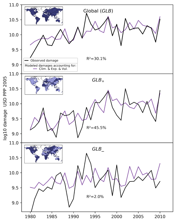
Reported global damage (black) from NatCatSERVICE for the entire globe and subregions of increasing and decreasing discharge in comparison to the damages simulated by our full model accounting for changes in climate, exposure and vulnerability. R² as the square of the Pearson-correlation coefficient denotes the explained variance achieved by the modeling approach.

---

FIG 6 / Image source: Sauer et al. (2021)

In some regions the explanatory power of our full model is even higher (see purple lines in Figure 7 and the explained variances given in each panel). In particular in the US it is surprisingly high reaching more than 80% in the region as a whole and in the regions with decreasing discharge. On the other hand there are regions where the explanatory power is very low. In our study we were not really able to explain these regional differences. This will be a long-term process including different steps such as validating the accuracy of the flood modeling chain by comparing them to observed flooded areas from satellite data (Mester et al. 2021 (under review)), validating exposure modeling in different areas, assessing the amount of underreporting in damage records in different world regions, resolving regional differences in empirical damage functions and improving knowledge on implemented protection standards. For this study we were really happy about the high agreement in the US which indicates that the general model approach makes sense and may depend more on regionally varying quality of asset maps or observational data rather than on the general physical representation of flooding as implemented in the hydrological models. For the attribution we decided to restrict statements to regions where the explanatory power of the model reaches at least 20% (grey panels in Figure 7).

---

Comparison observed damage time series from NatCatSERVICE (black, DObs) with modeled damages when accounting for changes in climate, exposure, and vulnerability (DFull, purple) for the nine world regions (left panel), as well as their subregions with homogeneous positive and negative trends in river discharge (middle and right panels). Explained variances R2 are derived from the Pearson correlation coefficients between damages DFull and DObs. Gray background colors highlight the regions where the explained variance of the full model is higher than 20%.

---

FIG 7 / Image source: Sauer et al. (2021)

So what is the pure effect of climate change on damages and what is the contribution of the other factors?

In order to understand the causes for changes in the damage trend and to quantify the contribution of climate and socio-economic changes, we can run the new model now in 3 different modes:

1. Full run: we start in 1980 and let all three components change over the years until 2010.
2. Run with fixed vulnerability: we let the climate and the exposure change over time, but keep the vulnerability at 1980 levels.
3. Pure climate change run: we let the climate change, but keep the vulnerability and exposure of the year 1980.

In Figure 8, the blue line (III) then shows how damage would have developed if only climate had changed since 1980 and all the human factors (population size, value of buildings, etc.) would have remained as they were in 1980. The orange line shows how damages would have been without any change in vulnerability e.g., without adaptation. The purple line shows the full run and aims to capture the observed damage.

By comparing the outcomes of the three modes, it is possible to quantify the contribution of each driver to the overall trend in damage: Climate-induced trends in damages (C) are estimated from the trend in the pure climate change run (III). Damage trends induced by changes in exposure (E) are then estimated from the difference between the trend in the pure climate change run (III) and the trend derived from an extended model additionally accounting changes in exposure (II). Finally, damage trends induced by changes in vulnerability (V) are estimated from the difference in trends between the fixed vulnerability run (II) and the full model (III):

$C = \frac{\alpha_{1980}}{D}$

$E = \frac{\alpha_{CliExp} - \alpha_{1980}}{D}$

$V = \frac{\alpha_{Full} - \alpha_{CliExp}}{D}$

$N = \frac{\alpha_{Obs}}{D}$

$M = \frac{\alpha_{Full}}{D}$

The equations above denote the absolute trend in the damage time series. To gain the contributions of each individual driver (C, E, V) and the overall observed (N) and modeled trend (M), the trends are normalised to the baseline damage D. We define the baseline damage as the annual reported mean damage the region experienced between 1985-2010.

And that is what we find on global scale:

---

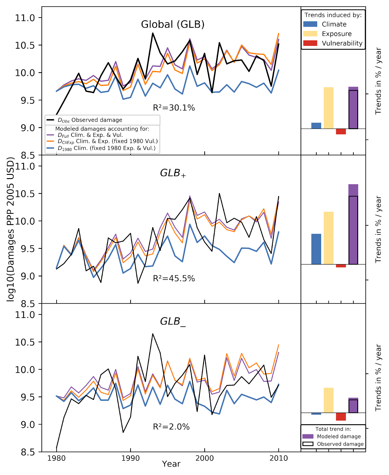
Observed and modeled time series of global river flood damages (1980-2010). Time series of observed damages from the NatCatService database (black) as well as modeled damages (multi-model median) when we run the model in three different modes: I) we let climate, exposure and vulnerability change over time (purple), II) we change climate and exposure (orange) keeping vulnerability at 1980 conditions, and III) we let only climate change and keep exposure and vulnerability on 1980-fixed levels. Bars indicate the relative trend in annual modeled (purple) and observed damages (black frames) and the individual contributions of each driver: climate (blue), exposure (yellow), vulnerability (red) relative to the recorded annual mean damage of the baseline period 1980-1995.

---

FIG 8 / Image source: Sauer et al. (2021)

Regarding the contributions of different drivers, for the entire globe we don’t see a significant contribution from climate (blue bar) to the overall damage trend (purple bar) (Figure 8a). The increasing trend in damages that we see roughly corresponds to the increase in the exposure, as the slightly small increase caused by climate is compensated by a small vulnerability reduction (red bar). In the R₊ regions of the globe (Figure 8b) this looks quite different. The climate contribution here is significant and also considerable in magnitude compared to the exposure contribution. For the R_- region the climate contribution was rather negative, but insignificant, although we do not have high confidence in the result due to the low explanatory power. However, this result highlights that when we want to assess climate contributions to damages we need to take a closer look. Globally, damages have not significantly increased due to climate change between 1980 and 2010, in many areas of the world climate has been an important contributor to changes in damages and in these areas the contribution was both significant and relevant in magnitude compared to the exposure trend.

What about the different subregions?

Similar to the results for the global land area and its subregions with increasing or decreasing changes in discharge, there are some large-scale world regions where our model shows a relatively high explanatory power (explained variance > 20%) and the climate signal also becomes significant as soon as you split them up according to positive or negative trends in discharge. These trends are mostly significantly positive (e.g. in parts of Latin America (LAM₊) and Eastern Asia (EAS and EAS₊)), but there are also areas with significant decreases e.g areas of Oceania (OCE_-) (Figure 9). In most regions e.g in Latin America and Eastern Asia, we see that climate has significantly increased damages in one subregion, but decreased damages in other regions (Figure 9). The contributions of climate to changes in damages are often insignificant and close to zero when we look only at the world regions as a whole or on the globe. Figure 9 shows us that looking only at entire world regions (blue dots) hides effects of changing climate as it often has significantly reduced or increased the damages.

---

---

What is the climate contribution compared to other drivers in the different world regions?

Our model also allows us to estimate the contribution of the other drivers. In general, our study confirms studies that found that increasing exposure was the most relevant driver. When we look at the small left panels in Figure 10 we can also generally state that exposure increase was the driving force between 1980-2010 and that climate contributions were only minor in comparison (SSA is an exception, but here we have low confidence in the model) as long as we do not split the world regions according to the trends in historical annual maximum discharge. It is once again important to look at the smaller world regions. Although still smaller than the exposure component, it is definitely no longer negligible. This is also the case in LAM₊, CAS₊, EAS₊ and SEA₊. In SEA₊ the climate was even the major driver.

In regions such as LAM and EAS the vulnerability reduction was indeed remarkable, but there are other world regions where it seems to have barely changed or even increased. Note, that vulnerability is usually assumed to decrease with time, as people learn to adapt. Here we find that in some regions and subregion vulnerability has increased, e.g in SEA, but also in developed regions such as NAM and OCE.

---

Contributions of changes in climate, exposure, and vulnerability to damages induced by river floods (1980-2010). Bars indicate the relative trend in annual modeled M (purple) and observed damages N (black frames) and the individual contributions of each driver: climate C1980 (blue), exposure E (orange), vulnerability V (red) relative to the recorded annual mean damage of the baseline period 1980-1995. From left to right, we present the trends in the entire world regions (R), and the subregions with positive (R₊) and (negative, R_-) discharge trends (see small maps). Grey background colors highlight the regions where the explained variance of the full model is higher than 20%.

---

FIG 10 / Image source: Sauer et al. (2021)

How certain are we and what needs to be done for further confirmation?

Of course, it would be really great if we could get a better understanding of the reasons for the low explanatory power of our model in some regions as that would probably help to improve our attribution tool for these regions. Potential reasons for the limited agreement between our model simulations and the observations in some regions are the following.